Gap Analysis
This example explains the procedure that is necessary to analyse a gap (e.g.
a superconducting gap) from an ARPES spectrum with arpys.
Throughout the example we will assume that we have a file ‘spectrum.p’
containing the ARPES spectrum and ‘gold.p’ with the corresponding gold
reference data, and that they have been loaded with
load_data() and saved as D and G
respectively.
Also, the dataloading and postprocessing modules have been loaded:
from arpys import dl,pp
1. Adjust Fermi level
First off, we need to precisely determine the Fermi level (which can vary
across angular channels).
This is done by fitting a Fermi-Dirac distribution convoluted by a Gaussian
to simulate the instrument resolution to each EDC.
Often it helps to add some additional linear components to the fit function,
as is done in fermi_fit_func().
1.1 Fermi fit
This process is automated in fig_gold_array()
(the more convenient method of using fit_gold()
relies on a specific organization of the data within G and is therefore
less recommended).
If we know that the energies lie along G.xscale and the shape of
G.data is (1, n_angles, n_energies) we would do:
levels, sigmas, slopes, offsets, functions = pp.fit_gold_array(G.data[0],
                                             G.xscale, ef, T)
where ef is a starting guess for the Fermi level and T is the
temperature at which the spectrum was taken.
Note
If the shape of G.data differs from the above, we would need to
reorganize it first. Ultimately,
fit_gold_array() expects a 2d array of shape
(n_angles, n_energies).
Confer the documentation of fit_gold_array() for
explanation of its output.
You will mostly need the levels only, but all the other output is useful
for checking whether the fit worked reasonably.
Note
You may notice that the execution of the above command may take some
time.
This is because there are n_angles fitting procedures that need
to be carried out.
If you have confirmed that the fitting worked reasonably well, it is
therefore a good idea to store the result in some form, and just load it
in again, whenever needed, instead of always carrying out the fit.
One way of achieving this is by using pickle:
import pickle
with open('my_file_to_store_gold_fit_results.p', 'wb') as f :
   pickle.dump(levels, f)
The levels can then be loaded by:
with open('my_file_to_store_gold_fit_results.p', 'rb') as f :
   levels = pickle.load(f)
Of course you can store more than just the levels.
This is a nice way of storing arbitrary python objects (however, some
objects cannot be pickled, like for example the functions).
arpys provides two convenience functions to save you some typing:
dump() and load_pickle().
1.2 Smoothing
Since the levels are usually quite noisy, it is recommended to apply some
operation to get a nicer curve. One way is to smoothen it (e.g. using
arpys.postprocessing.smooth()) or to fit a polynomial to the levels.
The following figure shows what this could look like.
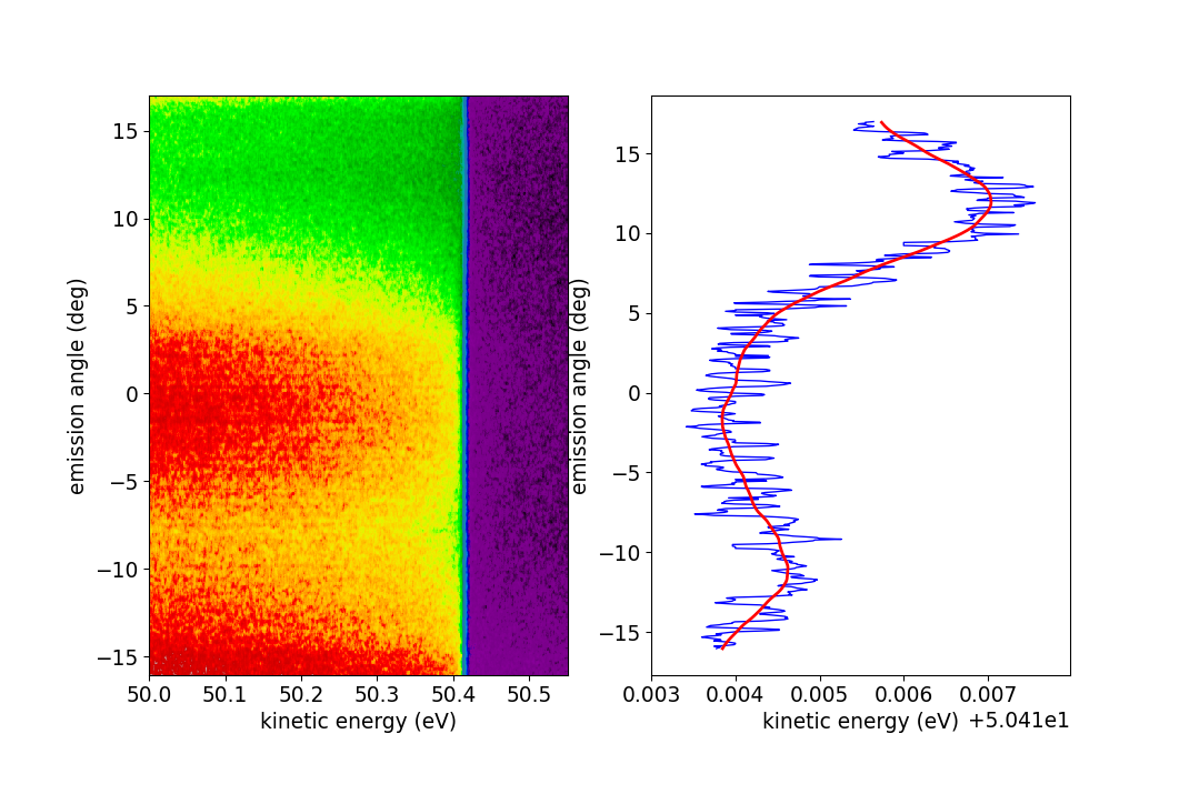
Fermi level fitting. To the left we see a false color plot of the gold
spectrum. Clearly the Fermi level is closely above 50.4 eV, which is what
was given as the starting guess for
fig_gold_array().
To the right, the resulting levels are plotted against the angles
(G.xscale in this example) in blue. Clearly, this result is rather noisy.
The red line shows a smoothed version of the blue curve.
1.3 Applying to data
Once we have our levels, we can use them to straighten our Fermi level in
the spectrum.
If we just want to plot the data, we can apply the levels continuously,
with the helper function adjust_fermi_level(),
which returns an energy mesh of shape (n_energies, n_angles) that can be
given to the pcolormesh() function.
However, if we are interested in further analysis (which we are in this
example), we need to apply the energy shifts discretely, in pixel units (the
follwoing assumes the same structure of D as we had for G before and
levels is the smoothened result of section 1.2 Smoothing):
pixel_shifts = pp.get_pixel_shifts(G.xscale, levels)
data, cutoff = pp.apply_pixel_shifts(D.data[0], pixel_shifts)
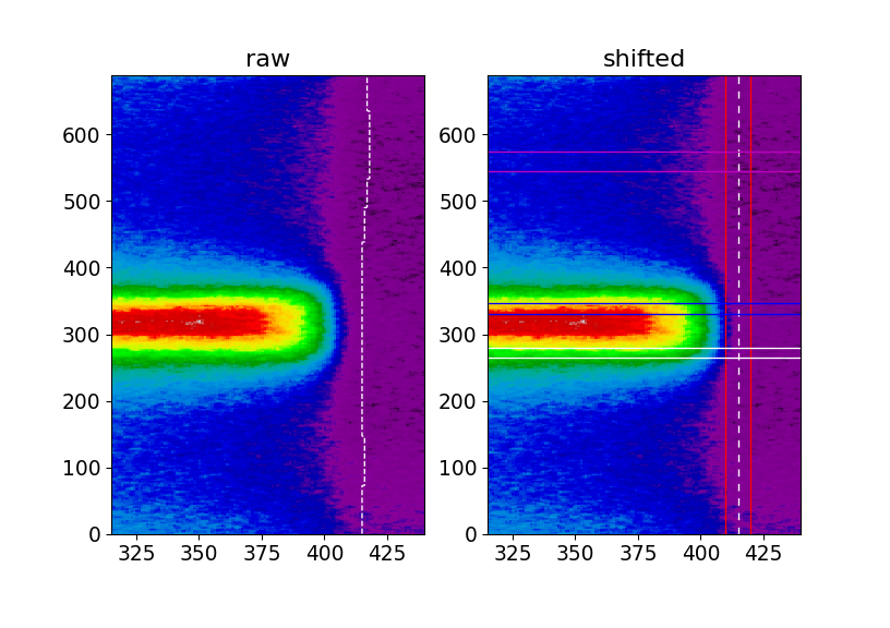
Application of the Fermi level correction. Left (raw) we see a part of our spectrum plotted in pixel coordinates with the curvy Fermi level indicated by the white dashed line. Right (shifted) the Fermi level has been adjusted and the white dashed line is straight. The red lines indicate the integration regime we will use for MDC extraction, the magenta lines show where we extract our background EDC from and the blue and white horizontal lines show where the actual EDCs at \(k_\mathrm{F}\) are taken from.
2. Finding \(k_\mathrm{F}\)
As a next step, in order to extract the EDCs at \(k_\mathrm{F}\), we need
to find it (them, actually, as there is one to the left and one to the right
in this example) by fitting Lorentzians to the MDC at \(E_\mathrm{F}\).
Useful functions in that context are
indexof() to get the index of the Fermi energy,
lorentzian() and of course scipy’s
scipy.optimize.curve_fit().
Note
At this point you can of course work in pixel, angular or k coordinates,
your choice.
Be reminded of arpys.postprocessing.angle_to_k() for the conversion
to k space.
The details of the fit can be left up to you. It can be helpful to try fitting only the relevant region along k, as can be seen in the figure, where the fit only considered the region where the black lines are drawn.
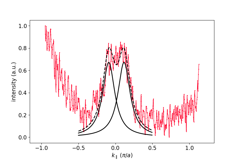
Extracted MDC and fitted Lorentzian curves.
3. EDC extraction and processing
Now that we know \(k_\mathrm{F}\), we can extract the EDCs from the data (as indicated in the figure above), subtract background and symmetrize.
3.1 Background subtraction
Of course, different situations may require different treatments of the background. Here are two common possibilities:
- Extract an EDC in a band-free region of the data, possibly smoothen it and use that as the background.
subtract_bg_matt(). A simple and intuitive method that has proven useful.
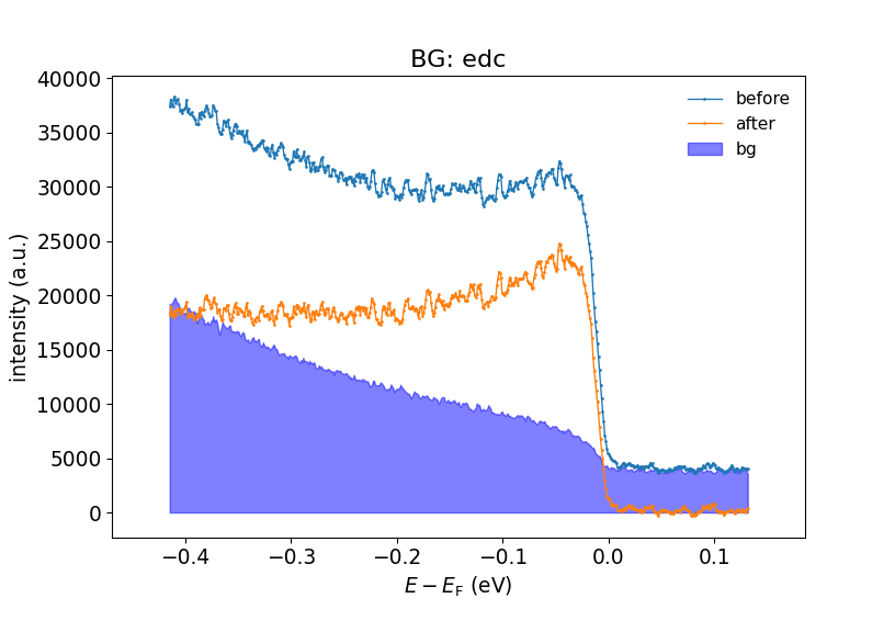
Background subtraction. Here the simple EDC subtraction method is used.
3.2 Symmetrization
Finally, you can use arpys.postprocessing.symmetrize_linear() to
symmetrize the EDC around \(E_\mathrm{F}\):
sym_edc, sym_energy = pp.symmetrize_linear(edc, ef_index, energies)
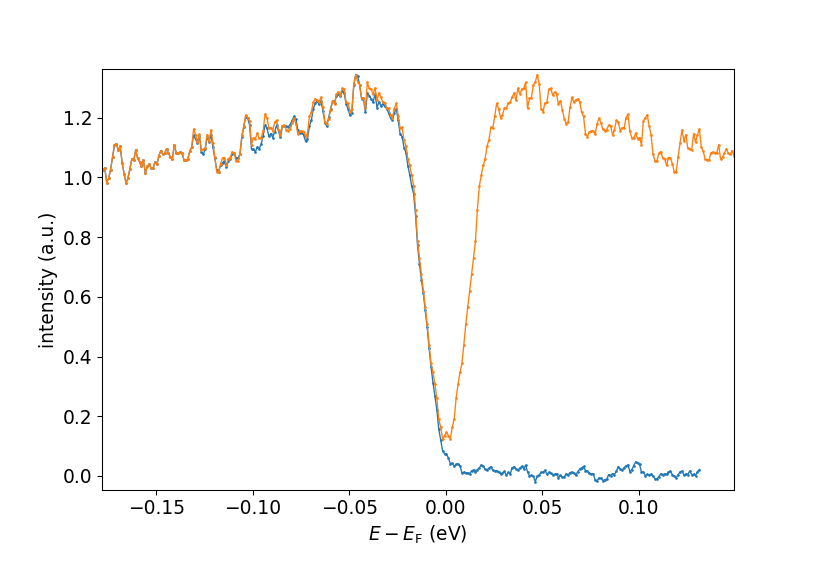
Original (blue) and symmetrized (orange) EDCs.